Tests of significance : Hypothesis, Null & Alternative, simple & Composite, Type I & Type II Errors, Critical Region, Critical Values, Level of Significance, Test, Test statistic One tailed & Two tailed , p- value, power of the test

Tests of significance

A very important aspect of the sampling theory is the study of the tests of significance. By tests of significance, we decide on the basis of sample results if the deviation between the observed sample statistic and the parameter value or the deviation between two independent sample statistics is significant or insignificant (due to chance or sampling fluctuations).

Hypothesis

A definite statement about the population parameter is called as hypothesis. (A hypothesis is a claim to be tested). For ex: a particular scooter gives average of 50 km per liter, proportion of unemployed persons is same in two different states, average life of an article produced by company A is greater than company B.

Null Hypothesis

A hypothesis of no difference is called null hypothesis. OR Null hypothesis is the hypothesis which is tested for possible rejection under the assumption that it is true (Prof. R. A. Fisher). For example, in case of a single statistic, H₀ will be that the sample statistic doesn’t differ significantly from the parameter. i.e. H₀:μ =μ0 and in the case of two statistic H₀ will be that the sample statistics don’t differ significantly i.e. H₀: µ₁₌µ₂.

Choice of null hypothesis

i) A hypothesis whose faulty rejection is more harmful. i

μi) ii) A hypothesis under which, we can find the probability distribution of test statistic.

Alternative Hypothesis

Any hypothesis which is complementary to the null hypothesis is called an alternative hypothesis. It is denoted by H_1.For example, if H₀: μ =μ0 i.e. the population has a specified mean µ₀, then the alternative hypothesis could be

i) H₁: μ ≠ μ0( μ < μ0orμ > μ0) ii) H₁: μ < μ0iii) H₁ : μ > μ0

The alternative hypothesis in (i) is known as a two sided(tailed) alternative while in (ii) & (iii) are known as (one sided alternatives) right tailed & left tailed alternative respectively.

Simple and Composite Hypothesis

A statistical hypothesis which completely specifies the population is called as simple hypothesis and the hypothesis which does not specifies the population is called as composite hypothesis. For ex: If x₁, x₂,----, x_n is a random sample from normal distribution with mean μ and variance б2 ,

then H₀: μ =μ0 and б2 =б02 is a simple hypothesis and each of the following is a composite hypothesis.

i) H₀: μ =μ0 ii) H₀: б2 =б02 iii) H₀: μ =μ0 & б2>б02 iv) H₀: μ =μ0 & б2<б02

v) H₀: μ <μ0 & б2 = б02 vi) H₀: μ >μ0 & б2 = б02 vii) H₀: μ >μ0 & б2 < б02

Errors in sampling

In sampling theory, we are liable to commit the following two types of errors. For example, in the inspection of a lot of manufactured items, the inspector will choose a sample of suitable size and then take decision whether to accept or reject the lot. In this case two errors are possible, one is rejection of a good lot and other is acceptance of bad lot. In testing of hypothesis these errors are called as type I & type II errors.

Type I error: Rejecting H₀ when it is true.

Type II error: Accepting H₀ when it is false (Accepting H₀ when H₁ is true).

If P [Reject Ho when it is true] = P [Reject Ho/ Ho] = α

and P [Accept Ho when it is wrong] = P [Accept Ho/ H₁] = β , then α and β are called the sizes of type I error and type II error respectively.

Thus in practice,

P P [Reject a lot when it is good] = α and P [Accept a lot when it is bad] = β

and α are β called the ‘Producer’s risk’ and ‘Consumers risk’ respectively.

The four types of decisions are shown in a table as follows.

Actual Situation	Decision
Actual Situation	Reject Ho	Accept Ho
Ho is true	Type I error	Correct decision
Ho is false	Correct decision	Type II error

Critical Region

A region corresponding to a statistic t in the sample space S in which Ho is rejected is called as critical region or region of rejection. If t = t (x₁, x₂,----, x_n ) is the value of the statistic based on a sample of size n , then

P ( t ∈ W / Ho ) = α and P ( t ∈ W' / H₁ ) = . β We have W U W' = S and

Wก W' = ф . ( W = rejection region & W = is acceptance region ).

Level of significance( l. o. s.)

The probability ‘α’ that a random value of the test statistic ‘t’ belongs to the critical region under Ho is known as ‘level of significance’. i.e. the size of the type I error is the level of significance.

Usually they are 5 % and 1% . The level of significance is always fixed in advance.

Interpretation: Proportion of cases in which Ho is rejected though it is true.

Critical values or significant values

The value of test statistic which separates the critical (rejection) region and acceptance region is called the critical value or significant value. It depends upon,

i) The level of significance used and

ii) The alternative hypothesis whether it is two tailed or one tailed.

Test: A rule which leads to the decision of rejection or acceptance of Ho.

Test Statistic: A function of sample observations which is used to test Ho is called is called as test statistic.

One and Two Tailed Tests:

The test, in which the alternative hypothesis is two tailed, is called two tailed test. For ex: H₀: μ =μ0and H₁: μ ≠ μ0.While the test, in which the alternative hypothesis is one tailed (right or left) is called one tailed test.

For ex: H₀: μ =μ0and H₁: μ > μ0. ( one tailed or right tailed test).

H₀: μ =μ0and H₁: μ < μ0. ( one tailed or left tailed test).

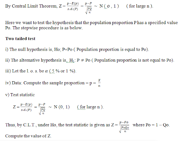
p- value (observed value of level of significance)

It is the smallest level of significance for which Ho would be rejected. If Z is the test statistic and Zo be its value under Ho for a given data set then P ( | Z | > | Zo | ) will be p-value. ( If Ho is accepted then p > α otherwise p < α ).

***

Procedure of testing of hypothesis

Any test of hypothesis is a stepwise procedure that leads to rejection or acceptance of the null hypothesis on the basis of samples drawn from the population.

The steps are as follows: i) Set up the null and alternative hypothesis (Ho and H₁). ii) Choose the appropriate level of significance. iii) Choose the appropriate test statistic Z/T and find its value. iv) Determine the critical values and critical region corresponding to level of significance and the alternative hypothesis (Zα or Zα/2 ). v) Conclusion: We compare the calculated value of Z or | Z |, with the tabulated value of Zα or Zα/2 . (For symmetrical distribution).

If | Z | _Cal ＜ Zα/2 (tab), accept Ho and conclude that there is no significant difference at (for two tailed test).

If | Z | _Cal ＞ Zα/2(tab), reject Ho and conclude that there is significant difference at (for two tailed test).

Similarly for one tailed test (left) If Z _Cal_＞ Zα (tab) , accept Ho and conclude that there is no significant difference at α % level of significance and if Z _Cal_＜ Zα (tab), reject Ho and conclude that there is significant difference, at α % level of significance.